The speaker enclosure and drivers are subject to variations in production, which may cause an imperfect match between the left and right speaker and thus lower IACC values. However, digital crossovers can be designed and adjusted in Acourate. It is therefore possible to correct the crossover for each driver inn each enclosure separately, so that the output from corresponding left and right drivers match each other as closely as possible and so that the drivers' output matches the intended crossover curve as closely as possible.

At this step we are not trying to correct the influence of the room or speaker placement. That will come later.

We need to use a suitable LogSweep covering the frequency range over which we want to linearize the crossover, but with the microphone picking up only the direct sound of the driver, not reflections from the room. It would be ideal to make the measurement in an anechoic chamber, or outdoors in an open field with the speaker pointing upwards and the baffle level with the ground. As it is rarely possible to make such an ideal measurement, we can try to minimize the influence of the room as much as possible. This can be done with the microphone about 30-50cm from the speaker. For high frequencies at that distance the room influence is reduced (and reflections typically have reduced high frequency content). As room influences can never be completely excluded, there is also the possibility, for example of making the measurement directly at the listening position and selecting the values ​​at Frequency Dependent Windowing wisely (meaning likely small values which will lead to smoothed corrections).

It is hard to make general recommendations as the properties of the sound field in different listening rooms are too complex. Opinions are contradictory as to whether it is helpful to linearize woofers below 200Hz (assuming one doesn't have the option of an anechoic chamber or of burying the speaker outdoors up to the baffle) as it is almost impossible to reduce room influences sufficiently. Therefore it would be expedient for you to try the various options for creating and editing of LogSweeps and observe the result in the changing IACC value and corresponding listening comparisons. Good Luck!

Load pulse response in Curve 1
Curve 1 using FDW> Curve 2
Mark the range to be linearized
Phase Extraction of highlighted area (minimum phase)> Curve 3
Amplitude inversion> Curve 4
Load original crossover in Curve 5
Convolution of inverted measurement (Curve 4) with original crossover (Curve 5) > Curve 6
delete content from Curve 2, select curve 6
Cut 'N Window of Curve 6 > Curve 2
Normalization of curve 2 (Individual Gain)
Save Curve 2 as new XO … ..dbl file

Detailed Instructions:

====

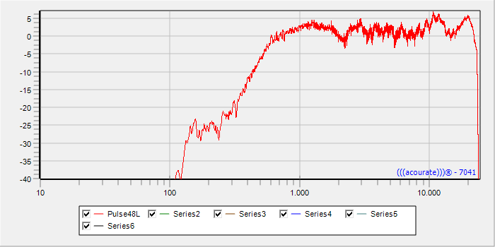
1. First, an impulse response has to be created by above-mentioned methods. Load this in curve. 1

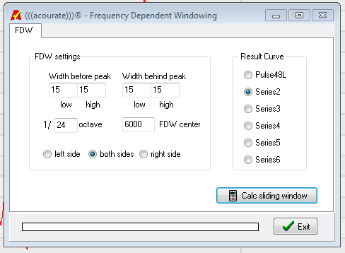
2. Select the tab TD-function> Frequency Dependent Windowing. The values ​​are to be adapted to the circumstances when creating the logsweeps used. Higher values ​​create more bumps in the frequency response, but include more room reflections. Smaller values ​create smaller andd more gradual corrections, but hide the room contribution better. Remember that the cutoff of room refllections is frequency-dependent (see FDW) and can be set differently for low and high frequencies. Save result in Curve 2.

3. In curve 2 mark the frequency range you want to correct with the two mouse buttons.. This may be the region having particularly large fluctuations or you can cover the full range of the crossover. At the beginning and end of the curve, however, some distance should be allowed, since these areas are affected by the windowing (FDW). (Therefore it is best that the logsweep cover a larger range than you want to use in correction.)

4. In the right pane of the amplitude window, the start and the end frequency are displayed as MarkR and MarkL, here 639Hz and 19396Hz.

5. To neutralize the curve outside of the marked area TD-Functions Phase Extraction is applied now. The amplitude above and below the selected frequencies is straightened. Select as the result curve Series3.

6. Invert the target curve into Serwies4 ith the FD-Functions> amplitude inversion.

7. You should get a screen similar to the screen above. Up to now, 4 curves are occupied, the last curve INVERS3 is active. Now, select the radio button for the still empty curve 5 and load the originally created crossover (with the name in the format XO___.dbl).

8. Now with TD-Functions> Convolution convolve the Invers3 curve with the original crossover file XO_.dbl and load in curve. 6 Now all curves are occupied. Select the radio button for Curve 2and delete it from the view. Then select curve 6 as the active curve.

9. As a result of the convolution, the number of samples has doubled in filter curve 6. The filter should be cut to the standard length of 65536 samples again. For this purpose select the TD functions> Cut'n Window tab and run with the settings shown here using as destination empty curve 2.

10. In the figure above, you can see the original crossover and the one you just created. Now the maximum amplitude must still be adjusted to the maximum amplitude of the original crossover:

11. In TD-Functions tab select> Normalization. The curve that should be normalized is No.2, choose individual gain. (Note: In this step it is important to note which crossover type is linearized, since not all crossovers, like the Neville Thiele crossover used in this example are normalized to 0dB. When other types of crossovers are used you may have to normalize to a different maximum amplitude by setting “normalization gain” appropriately (Max value among bins in the data window).

12. Now the preparation of the linearized crossover is complete. Save the current curve No.2 to a new folder under the old name of the crossover.

3. To test the linearized crossover carry out the measurement with the microphone in the same place as it was during the first LogSweep. Instead of the original crossover, the new linearized crossover is included after conversion to a * .wav file in the filter box, before recording in the LogSweep recorder.

4. The final check is carried out after the merging of all the linearized crossovers to a new multi-way .wav file. This is followed by another LogSweep at the listening position, which generates the pulse responses for the final filter creation. If the audible result of this final correction is unsatisfactory or the use of the linearized crossovers results in lower IACC values than before the linearization, a new linearization should be tried with other presets or microphone positions (see introductory text at the top of this article).